Regression Explained: A Practical Guide for Tax and Finance Teams
In the last post, I outlined how tax analytics has evolved — from deterministic rules in spreadsheets, through statistical thinking and machine learning, to generative AI. That post was deliberately broad: a map of the landscape before we start walking through it. This post takes the first real step into statistical territory by exploring regression — arguably the most widely useful analytical technique that most tax teams have never formally applied.
Regression sits in the statistical layer of the analytics stack. It’s the natural next step beyond the rule-based comparisons that dominate tax work today. Where a rule says “flag anything over £10,000,” regression asks “given everything we know about this transaction, what should the value be — and how far off is it?” That shift from fixed thresholds to data-driven expectations is what makes statistical thinking powerful, and regression is where it starts.
Why Understanding the Theory Matters More Than Ever
Before we get into the mechanics, it’s worth addressing something that has changed dramatically in the past two years.
The tools to implement regression — and many other analytical techniques — have become remarkably accessible. Python libraries handle the heavy lifting in a few lines of code. Low-code platforms offer drag-and-drop model building. And LLMs like Claude or ChatGPT can generate working regression code from a plain-English description of what you want to do.
This is genuinely transformative. Where previously there was a steep learning curve — understanding the syntax of specialist libraries, debugging obscure error messages, navigating documentation written for data scientists — the barrier to implementation has collapsed. A technically minded tax professional with a clear idea of what they want to achieve can now get working code in minutes rather than weeks.
But there’s a problem: if you don’t understand what the tool is doing, you can’t tell when it’s giving you the wrong answer.
If we’re going to use these techniques — and we should — then we need to understand what they’re doing. Not because we need to derive the mathematics by hand, but because we need to know which technique fits which problem, what the outputs actually mean, what the assumptions are, and where the method breaks down. If an LLM generates regression code for you, you need to be confident that it’s the right approach, that the results are sensible, and that you can explain what you’ve done to a tax director, an auditor, or a regulator.
The risk isn’t that the code won’t run. It’s that it will run, produce a number, and nobody in the room knows whether to trust it.
That’s what this post aims to address. I’ll explain regression from the ground up — what it is, how it works conceptually, and where it applies in tax and finance — so that when you do use an LLM or a library to build one, you’re working from a position of understanding rather than faith.
What Is Regression?
At its core, regression answers a simple question: how does one thing change when another thing changes?
More precisely, it finds the mathematical relationship between a variable you want to explain or predict (the dependent variable, often called y) and one or more variables you think influence it (the independent variables, or predictors, often called x).
The output is an equation — a formula that describes how the predictors relate to the outcome. You can then use that equation to make predictions, identify anomalies, or understand which factors matter most.
Tax professionals already do a version of this intuitively. When you review monthly VAT returns and think “output VAT should be roughly 20% of revenue,” you’re carrying an implicit model in your head. Regression formalises that intuition, fits it to actual data, and quantifies how well it holds.
Building the Intuition: From Lines to Planes to Hyperplanes
The easiest way to understand regression is visually, starting with the simplest case and building up.
One Predictor: A Line
Imagine plotting your data on a scatter chart. Revenue on the x-axis, output VAT on the y-axis. Each dot is one period. If VAT is consistently around 20% of revenue, those dots will form a roughly linear pattern.
Simple linear regression draws the line of best fit through those points — the straight line that minimises the total distance between the line and every data point.
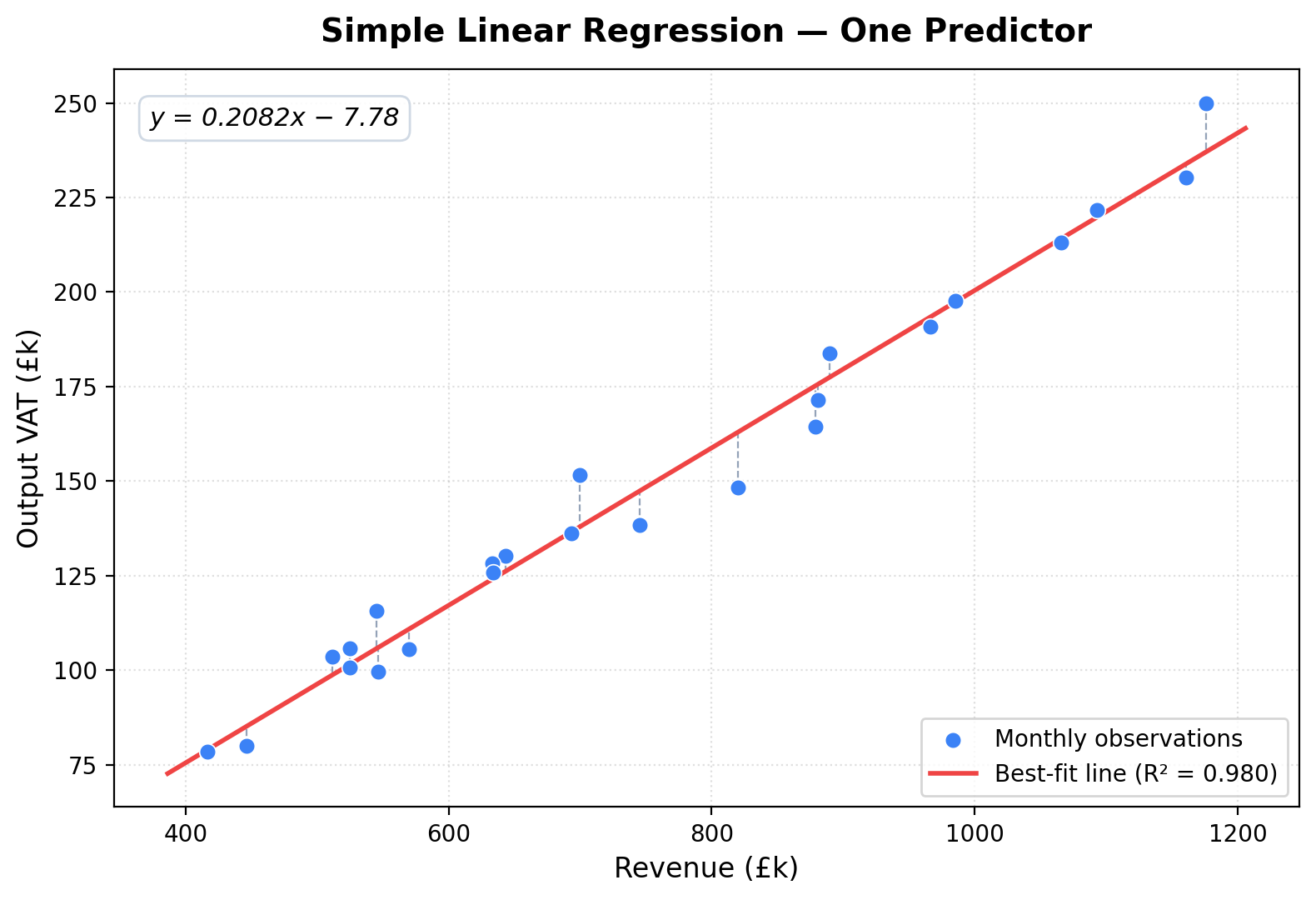
The equation of that line is:
y = β₀ + β₁x
Where β₀ is the intercept (where the line crosses the y-axis) and β₁ is the slope (how much y changes for each unit change in x). For our VAT example, you’d expect β₁ to be close to 0.20 and β₀ to be close to zero. If the line fits well, months where the actual VAT deviates significantly from the line are worth investigating.
Two Predictors: A Flat Surface
Now suppose you suspect that VAT isn’t just driven by revenue, but also by the mix of zero-rated and standard-rated sales. You have two predictors: total revenue and the proportion of standard-rated sales.
With two predictors, the regression doesn’t fit a line — it fits a flat plane through a three-dimensional scatter of points. Think of it as a tilted sheet of paper suspended in a room full of floating dots.
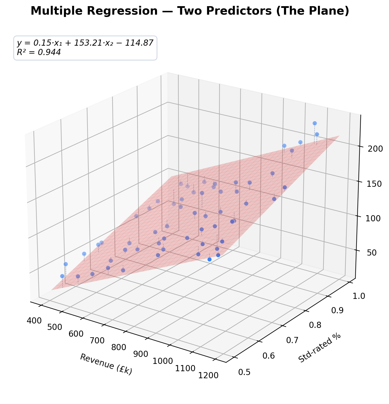
The equation becomes:
y = β₀ + β₁x₁ + β₂x₂
This is literally the equation of a plane. Each coefficient tells you how much VAT changes when that predictor changes, holding the other constant. The regression finds the plane that best fits the data — same principle as before, just in one more dimension.
Three or More Predictors: Hyperplanes
Add a third predictor — say, the volume of EU exports — and you’re fitting a hyperplane in four-dimensional space. The maths works identically, but this is where geometric intuition breaks down because we can’t visualise four dimensions. The equation simply adds another term:
y = β₀ + β₁x₁ + β₂x₂ + β₃x₃
Each additional predictor adds a term and a dimension. The fundamental idea — “find the surface that best fits the data” — stays the same throughout. This is why the line and plane examples are so valuable: they build the intuition you carry with you when the algebra moves beyond what you can draw.
In practice, tax regression models could use five, ten, or more predictors. The principle never changes. The model finds the combination of coefficients that produces the best-fitting surface through your data.
How Does Regression Find the “Best Fit”?
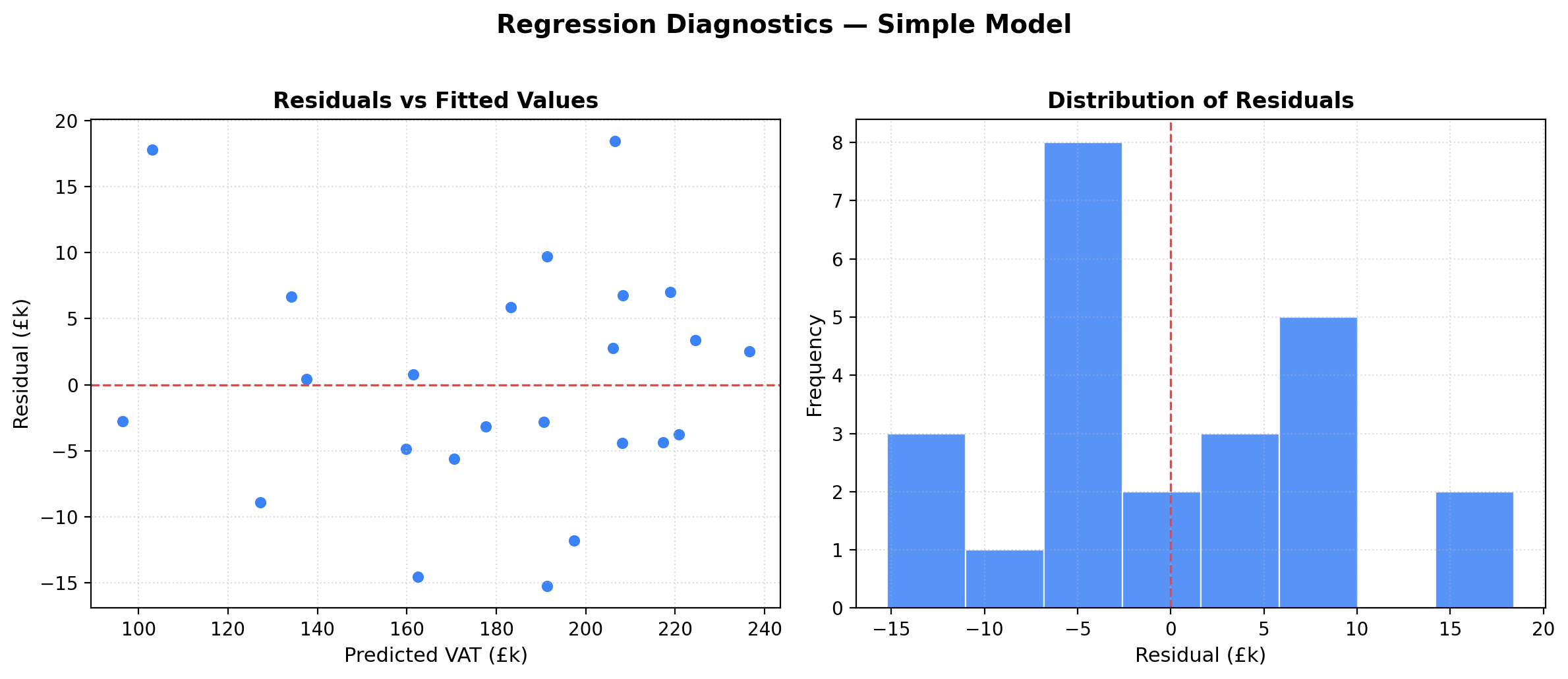
The most common method is called Ordinary Least Squares (OLS). The idea is straightforward: for every data point, measure the vertical distance between the actual value and the value predicted by the line (or plane, or hyperplane). Square each of those distances. Then find the line that makes the total of those squared distances as small as possible.
Why squared? Two reasons. First, squaring ensures that points above and below the line don’t cancel each other out. Second, it penalises large errors more heavily than small ones, which is usually what we want — a model that’s slightly off on most points is preferable to one that’s wildly wrong on a few.
The “residuals” — the gaps between actual and predicted values — are the heart of regression diagnostics. If the model fits well, residuals should be small and randomly scattered. If they show patterns (e.g., residuals that grow larger as values increase), that tells you the model is missing something.
Key Concepts You Need to Know
Before applying regression in practice, there are a few concepts worth understanding. You don’t need to memorise formulas, but you do need to know what these terms mean when you encounter them — in an LLM-generated output, a library’s documentation, or a conversation with a data scientist.
R-squared (R²)
R-squared measures how much of the variation in your dependent variable is explained by the model. It ranges from 0 to 1. An R² of 0.95 means 95% of the variation in output VAT is explained by the predictors. The remaining 5% is unexplained — noise, missing variables, or random fluctuation.
A high R² doesn’t guarantee the model is correct, and a low R² doesn’t mean it’s useless. Context matters. In a tightly controlled process like VAT on domestic sales, you’d expect R² above 0.90. In something more variable, like predicting transfer pricing adjustments across jurisdictions, R² of 0.60 might be excellent.
Coefficients and Their Interpretation
Each coefficient (β) tells you the expected change in the outcome for a one-unit change in that predictor, holding everything else constant. In a VAT model, if the coefficient on revenue is 0.19, that means each additional £1 of revenue is associated with approximately £0.19 of output VAT. If it should be 0.20, that small discrepancy might reveal systematic under-reporting or a data quality issue.
Statistical Significance (p-values)
A p-value tells you how likely it is that a predictor’s coefficient is different from zero just by chance. A low p-value (typically below 0.05) suggests the predictor has a genuine relationship with the outcome. A high p-value suggests the predictor may not be contributing meaningfully to the model.
In tax contexts, this helps you distinguish between predictors that genuinely drive the outcome and ones that are just noise. If you include the number of bank holidays in the month as a predictor of output VAT and it comes back with a p-value of 0.87, you can safely ignore it.
Overfitting
A model with too many predictors relative to the number of observations can start fitting the noise rather than the signal. It performs brilliantly on the data it was trained on but poorly on new data. This is called overfitting, and it’s a real risk when you have many potential predictors and relatively few periods of data — which is common in tax, where you might only have 24 or 36 monthly data points.
The antidote is simplicity: use the fewest predictors that explain the outcome adequately, and validate the model on data it hasn’t seen before.
Practical Tax Use Cases
Regression isn’t an academic exercise — it solves real problems that tax teams face. Here are several areas where it could apply directly.
VAT Reconciliation and Anomaly Detection
The most intuitive application: modelling the expected relationship between revenue and output VAT. A well-fitted regression gives you a data-driven expectation for each period’s VAT liability. Months where actual VAT deviates significantly from the predicted value — large positive or negative residuals — are flagged for review.
This is more sophisticated than a simple percentage check because the model can account for multiple factors simultaneously: revenue mix, zero-rated sales, credit notes, foreign currency effects. The residuals become your anomaly detection mechanism.
Transfer Pricing Benchmarking
Transfer pricing relies on demonstrating that intercompany transactions are priced at arm’s length. Regression is a standard tool in benchmarking studies — it can model the relationship between a company’s financial indicators (revenue, assets, headcount) and its profitability, then compare the tested party’s results to the model’s predictions.
Multiple regression is particularly useful here because profitability is rarely explained by a single factor. A model might include revenue, total assets, R&D intensity, and industry classification as predictors, producing a more nuanced benchmark than simple quartile analysis.
Expense Forecasting and Provision Estimation
Tax provisions require estimates of future tax liabilities, which in turn depend on forecasted expenses, revenues, and deductions. Regression on historical data can produce projections that account for seasonal patterns, growth trends, and the relationships between different expense categories — moving beyond flat-line extrapolations or simple growth rates.
Effective Tax Rate Analysis
An organisation’s effective tax rate (ETR) is influenced by many factors: geographic profit mix, permanent differences, incentives, prior year adjustments. Regression can decompose which factors contribute most to ETR variation across periods, helping tax teams explain movements to the board and identify the drivers of unexpected rate changes.
Cost Driver Analysis for R&D Tax Relief
For R&D claims, demonstrating that qualifying expenditure is driven by legitimate research activity is important. Regression can model the relationship between R&D headcount, project spend, and claimed relief — providing evidence that the claim is proportionate and consistent with the underlying cost drivers.
What Regression Doesn’t Do
It’s equally important to understand the boundaries.
Regression identifies associations, not causes. If your model shows that marketing spend is correlated with higher VAT liabilities, that doesn’t mean marketing spend causes VAT to increase — both are probably driven by revenue growth. Interpreting regression coefficients as causal without domain knowledge is a common and costly mistake.
Regression also assumes relationships are linear (in standard linear regression). If the true relationship is curved, kinked, or conditional, a simple linear model will miss it. There are extensions — polynomial regression, interaction terms, generalised linear models — but recognising when you need them requires understanding what the basic model assumes.
Finally, regression is sensitive to outliers. A single extreme data point can pull the entire line toward it, distorting predictions for everything else. Tax data is particularly prone to this: one-off adjustments, large intercompany settlements, or year-end true-ups can dominate the model if not handled carefully.
What Comes Next
This post has laid the conceptual groundwork. In the next post, I’ll move from theory to practice: building a working regression model in Python using the synthetic dataset we created earlier in this series. We’ll walk through the full workflow — loading data, selecting features, fitting the model, interpreting the output, and diagnosing problems — with code you can run and adapt.
The goal isn’t to make you a statistician. It’s to give you enough understanding that when you use an LLM to generate regression code, or when a data scientist presents you with a model, you know what questions to ask, what the numbers mean, and whether to trust the results.
The barrier to implementation has never been lower. The barrier to understanding remains exactly where it always was — and that’s the one that matters.