Can't Access Real Tax Data? Here's How to Create Synthetic Datasets That Work
This is the first “real” post after the launch, and starting with synthetic data feels right. I can’t (and won’t) share real corporate records, so everything I demonstrate will rely on realistic but artificial datasets. The aim is to create tax-shaped data that looks and behaves like what you’d expect in practice—transactions, vendors, VAT/tax fields, periods, and narratives—without exposing anything sensitive.
I’ll outline practical, Python-based ways to generate datasets that feel familiar to tax professionals and are useful for classification (e.g., deductible vs non-deductible), anomaly detection (unexpected spikes/dips), time-series analysis (seasonality and trends), forecasting (projecting VAT or expense lines), and regression (modelling relationships such as VAT vs revenue or cost drivers). Even if you don’t code, this should be useful to understand the art of the possible—and you’re very welcome to download the datasets I create and use them directly.
Next up, we’ll cover why synthetic data is especially valuable for tax technologists in industry.
Why Start with Synthetic Data
In every project, the first obstacle is the same: getting access to real data. We can’t share it externally, and even inside large organisations, obtaining access for early experimentation can take months. To demonstrate what’s possible, we often have to start without it.
Synthetic data solves this by giving us realistic examples that let us:
- prove a concept before touching production systems,
- work safely in non-secure or sandbox environments, and
- communicate value to stakeholders before governance and access are in place.
In short, synthetic data lets us move faster and more safely—a bridge between ideas and real implementation.
Why this matters: every successful analytics project begins with a believable dataset. When you can’t get one, you build it.
The Types of Data We Use in Tax (Structured vs Unstructured)
In tax, most day-to-day analysis runs on structured data: tidy, tabular exports with stable columns and types—think ledger and subledger lines, invoice headers and details in CSV, VAT return extracts, reference tables (FX rates, tax codes), and monthly or quarterly summaries. This is the data that flows cleanly into spreadsheets, notebooks, and BI tools, and it underpins core processes such as P&L reviews, deductibility checks, and VAT reconciliations.
Alongside that sits a large universe of unstructured information: invoices and contracts as PDFs or images, emails and approval notes, free-text narratives on postings, and semi-structured documents that don’t fit neatly into rows and columns. Historically this has been harder to tap, but that’s changing—OCR and intelligent document processing, computer vision, and LLM-assisted extraction are making these sources increasingly accessible; e-invoicing where adopted also delivers more structure out of the box.
For this post, we’ll stay with structured data because it’s what most tax controls rely on today and it’s straightforward to generate reproducibly—while recognising that much of the interesting context lives in unstructured sources we can return to later and use to enrich the synthetic tables.
Our Objective (and the Dataset We’ll Build)
To keep things concrete, we’ll generate a typical line-item transactions dataset—the kind a tax professional would export for reviews and controls. Think of it as “G/L-flavoured” rather than tied to any one system: familiar fields, familiar narratives, and enough variety to support classification, anomaly detection, time-series analysis, forecasting, and regression.
| Field (SAP Name) | Description | Data Type / Length | Example |
|---|---|---|---|
| BUKRS | Company code | CHAR(4) | GB01 |
| BELNR | Accounting document number | CHAR(10) | 1900001234 |
| GJAHR | Fiscal year | NUMC(4) | 2025 |
| BUZEI | Line item number | NUMC(3) | 001 |
| BUDAT | Posting date | DATS | 2025-09-30 |
| BLART | Document type | CHAR(2) | KR |
| WAERS | Document currency | CUKY(5) | GBP |
| KURSF | Exchange rate | CURR(9,5) | 1.00000 |
| WRBTR | Amount in document currency | CURR(13,2) | 1500.00 |
| DMBTR | Amount in local currency | CURR(13,2) | 1500.00 |
| HKONT | G/L account | CHAR(10) | 600000 |
| KOSTL | Cost center | CHAR(10) | MKT100 |
| PRCTR | Profit center | CHAR(10) | UK_SALES |
| ZUONR | Assignment number | CHAR(18) | PO-45001234 |
| SGTXT | Item text | CHAR(50) | Office supplies |
| AUGBL | Clearing document | CHAR(10) | 1900005678 |
| AUGDT | Clearing date | DATS | 2025-10-05 |
Section 1: Import Required Libraries
First, let’s import the standard Python libraries we’ll need for basic data generation:
# Standard Python libraries for basic data generation
import random               # For random number generation and sampling
import datetime as dt       # For working with dates and times
import pandas as pd         # For tabular data structures and analysis

# Set seed for reproducible results
random.seed(42)

print("✓ Standard libraries imported successfully")
print("✓ Random seed set to 42 for reproducible results")
✓ Standard libraries imported successfully
✓ Random seed set to 42 for reproducible results
Section 2: Generate Basic Data with Python
Let’s start with a simple Python approach to generate synthetic SAP-style transaction data. We’ll build this step-by-step, showing how you can create realistic-looking data using just standard libraries.
Why Start with Basic Python?
Before reaching for specialised libraries, it’s worth understanding what you can achieve with just Python’s standard library. This approach has several advantages:
- No dependencies - Works immediately with any Python installation
- Full transparency - Every line of code is visible and controllable
- Learning foundation - Understanding the basics makes advanced techniques clearer
- Good enough for many use cases - Simple randomisation works well for initial prototypes
The basic approach uses Python’s random module to sample from predefined lists and generate random values within specified ranges. We’ll create transactions that look structurally correct—proper field names, appropriate data types, realistic value ranges—even if the content is somewhat repetitive.
Let’s see how far we can get with just standard Python.
Step 1: Define Reference Data
First, we’ll set up the reference lists that we’ll sample from randomly.
What is Reference Data?
In any accounting or ERP system, reference data (sometimes called master data or configuration tables) defines the valid values and rules that govern how transactions can be recorded. These are the “controlled vocabularies” maintained by finance teams—lists of company codes, the chart of accounts, cost center hierarchies, currency codes, and document types. In SAP terms, this is the customising configuration that makes the system work for your specific organisation.
For synthetic data generation, reference data serves three essential purposes:
1. Ensures structural validity - Rather than generating arbitrary strings like “XYZ999” for a company code, we sample from a predefined list of valid codes (GB01, DE01, etc.). This means our synthetic transactions will pass basic validation checks and look structurally correct to anyone familiar with the domain.
2. Enables realistic distributions - By controlling which values appear in our reference lists, we can simulate real-world patterns. For example, if your organisation has 10 cost centers but 80% of expenses go through three of them, you can weight the random sampling accordingly. This creates datasets that mirror actual business operations.
3. Maintains field relationships - Reference data lets us build intelligent generation rules where related fields stay consistent. For instance, when we randomly select company code “GB01” (a UK entity), we can ensure the base currency is GBP, posting dates follow UK business day patterns, and amounts fall within typical UK expense ranges. Without reference data, these fields would be independently random and create nonsensical combinations.
In this basic Python approach, we’ll define simple lists and dictionaries for our reference data. Later, when we move to the Faker-enhanced approach, we’ll see how to build more sophisticated relationships between these reference tables to create truly realistic synthetic data.
# Set the number of transactions we want to generate
n_rows = 1000

# Create categories for the synthetic data fields from which to sample randomly
company_codes = ["GB01", "GB02", "DE01", "US01"]
document_types = ["KR", "KA", "ZP", "DR", "DG", "AB"]  # Vendor invoice, Asset posting, Payment, etc.
currencies = ["GBP", "EUR", "USD"]

# G/L Account ranges (UK tax-sensitive expense accounts only)
gl_accounts = {
    "600000": "Office Expenses",
    "610000": "IT & Software",
    "620000": "Travel & Subsistence",
    "625000": "Motor Expenses",
    "630000": "Entertainment - Client",
    "635000": "Entertainment - Staff",
    "640000": "Professional Fees",
    "650000": "Marketing & Advertising",
    "660000": "Training & Development",
    "670000": "Charitable Donations",
    "680000": "Bad Debts",
    "690000": "Depreciation"
}

cost_centers = ["MKT100", "FIN200", "IT300", "HR400", "OPS500"]
profit_centers = ["UK_SALES", "UK_ADMIN", "DE_SALES", "US_SALES"]

print("✓ Reference data defined")
print(f"  • {len(company_codes)} company codes")
print(f"  • {len(gl_accounts)} G/L accounts (all tax-sensitive expenses)")
print(f"  • {len(currencies)} currencies")
print(f"  • {len(cost_centers)} cost centers")
print(f"  • {len(profit_centers)} profit centers")
✓ Reference data defined
  • 4 company codes
  • 12 G/L accounts (all tax-sensitive expenses)
  • 3 currencies
  • 5 cost centers
  • 4 profit centers
Step 2: Generate Transaction Records
Now let’s generate the actual transactions by looping through and creating each record with realistic values:
# Initialize empty list to store transactions
transactions = []

# Generate n_rows transactions
for i in range(n_rows):
    # Generate document number (year + sequential)
    doc_year = random.choice([2024, 2025])
    doc_number = f"{doc_year}{i+1:06d}"

    # Generate posting date within the fiscal year
    start_date = dt.date(doc_year, 1, 1)
    end_date = dt.date(doc_year, 12, 31)
    days_between = (end_date - start_date).days
    posting_date = start_date + dt.timedelta(days=random.randint(0, days_between))

    # Select currency and calculate exchange rate
    currency = random.choice(currencies)
    if currency == "GBP":
        exchange_rate = 1.00000
    elif currency == "EUR":
        exchange_rate = round(random.uniform(0.85, 0.90), 5)
    else:  # USD
        exchange_rate = round(random.uniform(1.20, 1.30), 5)

    # Generate amount (expenses are negative)
    amount_doc = round(-random.uniform(50, 25000), 2)
    amount_local = round(amount_doc * exchange_rate, 2)

    # Create the transaction record as a dictionary
    transaction = {
        "Company Code": random.choice(company_codes),
        "Accounting Document": doc_number,
        "Fiscal Year": doc_year,
        "Line Item": f"{random.randint(1, 20):03d}",
        "Posting Date": posting_date.strftime("%Y-%m-%d"),
        "Document Type": random.choice(document_types),
        "Document Currency": currency,
        "Exchange Rate": exchange_rate,
        "Amount (Document Currency)": amount_doc,
        "Amount (Local Currency)": amount_local,
        "G/L Account": random.choice(list(gl_accounts.keys())),
        "Cost Center": random.choice(cost_centers),
        "Profit Center": random.choice(profit_centers),
        "Assignment Reference": f"REF-{random.randint(100000, 999999)}",
        "Item Text": "Basic transaction text",
        "Clearing Document": "",  # Clearing document (populated for some records)
        "Clearing Date": ""       # Clearing date (populated for some records)
    }

    # Add clearing information for 30% of transactions (simulating payments)
    if random.random() < 0.3:
        clearing_date = posting_date + dt.timedelta(days=random.randint(1, 30))
        transaction["Clearing Document"] = f"{doc_year}{random.randint(500000, 999999)}"
        transaction["Clearing Date"] = clearing_date.strftime("%Y-%m-%d")

    transactions.append(transaction)

print(f"✓ Generated {len(transactions)} transaction records")
✓ Generated 1000 transaction records
Step 3: Convert to DataFrame
Let’s convert our list of dictionaries into a pandas DataFrame for easier analysis:
# Convert to DataFrame
basic_df = pd.DataFrame(transactions)

print(f"✓ Created DataFrame with {len(basic_df)} rows and {len(basic_df.columns)} columns")
print("\nFirst 5 records:")
print(basic_df.head(5))
✓ Created DataFrame with 1000 rows and 17 columns

First 5 records:
  Company Code Accounting Document  Fiscal Year Line Item Posting Date  \
0         GB01          2024000001         2024       018   2024-01-13
1         US01          2024000002         2024       008   2024-10-14
2         DE01          2025000003         2025       004   2025-06-24
3         US01          2025000004         2025       003   2025-01-23
4         GB01          2024000005         2024       013   2024-05-28

  Document Type Document Currency  Exchange Rate  Amount (Document Currency)  \
0            KR               USD        1.22750                    -5619.11
1            DR               GBP        1.00000                   -17914.69
2            KR               EUR        0.85777                   -23932.47
3            DG               USD        1.24594                    -3164.41
4            ZP               GBP        1.00000                   -21390.18

   Amount (Local Currency) G/L Account Cost Center Profit Center  \
0                 -6897.46      670000       HR400      UK_SALES
1                -17914.69      670000       IT300      UK_SALES
2                -20528.55      640000      MKT100      DE_SALES
3                 -3942.66      630000      OPS500      DE_SALES
4                -21390.18      650000       IT300      UK_ADMIN

  Assignment Reference               Item Text Clearing Document Clearing Date
0           REF-131244  Basic transaction text        2024764951    2024-01-21
1           REF-895667  Basic transaction text
2           REF-988662  Basic transaction text
3           REF-705397  Basic transaction text        2025524025    2025-01-26
4           REF-488162  Basic transaction text
# Let's examine the basic data quality
print("Basic Data Generation - Quality Assessment:")
print("=" * 50)
print(f"Total records: {len(basic_df)}")
print(f"Date range: {basic_df['Posting Date'].min()} to {basic_df['Posting Date'].max()}")
print(f"Company codes: {sorted(basic_df['Company Code'].unique())}")
print(f"Currencies: {sorted(basic_df['Document Currency'].unique())}")
print(f"Cleared transactions: {basic_df['Clearing Document'].astype(bool).sum()} ({basic_df['Clearing Document'].astype(bool).mean():.1%})")

print("\nSample transaction text variety:")
print(basic_df['Item Text'].value_counts().head())
Basic Data Generation - Quality Assessment:
==================================================
Total records: 1000
Date range: 2024-01-01 to 2025-12-31
Company codes: ['DE01', 'GB01', 'GB02', 'US01']
Currencies: ['EUR', 'GBP', 'USD']
Cleared transactions: 300 (30.0%)

Sample transaction text variety:
Item Text
Basic transaction text    1000
Name: count, dtype: int64
Section 4: Generate Realistic Data with Faker
The basic approach works but has obvious limitations - the transaction text is repetitive and doesn’t look realistic. Let’s enhance this with the Faker library, which provides much more sophisticated data generation capabilities.
What is Faker?
Faker is a Python library that generates realistic fake data for a wide range of use cases. Instead of writing “Basic transaction text” a thousand times, Faker can produce convincing company names, addresses, dates, personal names, and much more—all localised to different countries and languages.
Why Faker Matters for Tax Data
In tax analytics, context matters. A transaction description that reads “Office supplies from ABC Corp in London” tells a richer story than “Basic transaction text”. When we later build classification models or anomaly detection systems, these realistic narratives provide the kind of signal that makes models generalise better to real-world data.
Faker also helps us:
- Generate locale-specific data - UK company names for GB entities, German names for DE entities
- Create realistic patterns - business day bias for posting dates, plausible vendor names
- Maintain reproducibility - seed the random generator to get the same “fake” data every time
- Scale effortlessly - generate thousands of unique, believable records without manual effort
Let’s see how to set it up:
# Import faker
from faker import Faker

# Create Faker instances for different locales
fake_en = Faker('en_GB')  # UK English
fake_de = Faker('de_DE')  # German
fake_us = Faker('en_US')  # US English

# Set seed for reproducible results
Faker.seed(42)

print("✓ Faker instances created for multiple locales")
print("✓ Faker seed set to 42 for reproducible results")
✓ Faker instances created for multiple locales
✓ Faker seed set to 42 for reproducible results
Now let’s create a much more sophisticated data generator using Faker. We’ll break this down step-by-step to show how Faker can produce realistic company names, addresses, transaction descriptions, and other contextual details.
Step 1: Set Up Enhanced Reference Data with Locale Intelligence
In the basic approach, our reference data was simple lists and dictionaries. Now we’ll enhance it by embedding business logic directly into the reference structures. The key difference: instead of just listing company codes, we’ll create a rich data structure that associates each company with its locale-specific Faker instance and base currency. This allows the generator to automatically adapt its behavior based on which entity is selected.
This is where the power of structured reference data really shines—when “GB01” is randomly chosen, the generator immediately knows to:
- Use the UK Faker instance for realistic British names and addresses
- Set GBP as the base currency
- Apply appropriate exchange rate logic for foreign transactions
Let’s define these enhanced reference structures:
# Enhanced company data with locale-specific Faker instances
company_data = {
    "GB01": {"name": "Analytax UK Ltd", "faker": fake_en, "currency": "GBP"},
    "GB02": {"name": "Analytax Holdings Ltd", "faker": fake_en, "currency": "GBP"},
    "DE01": {"name": "Analytax Deutschland GmbH", "faker": fake_de, "currency": "EUR"},
    "US01": {"name": "Analytax Corp", "faker": fake_us, "currency": "USD"}
}

# Document types with descriptions (expense-focused)
document_types = {
    "KR": "Vendor Invoice",
    "ZP": "Payment",
    "DG": "Credit Memo",
    "AB": "Asset Posting",
    "SA": "G/L Account Document",
    "KG": "Vendor Credit Memo"
}

# Enhanced G/L Account mapping with account type classification
gl_accounts_enhanced = {
    "600000": {"desc": "Office Expenses", "type": "Expense"},
    "610000": {"desc": "IT Expenses", "type": "Expense"},
    "620000": {"desc": "Travel & Entertainment", "type": "Expense"},
    "630000": {"desc": "Professional Services", "type": "Expense"},
    "640000": {"desc": "Marketing & Advertising", "type": "Expense"},
    "650000": {"desc": "Training & Development", "type": "Expense"},
    "700000": {"desc": "Salaries & Wages", "type": "Expense"},
    "710000": {"desc": "Social Security", "type": "Expense"},
    "800000": {"desc": "Depreciation", "type": "Expense"}
}

# Cost centers by function
cost_centers_enhanced = {
    "MKT100": "Marketing",
    "SAL200": "Sales",
    "FIN300": "Finance",
    "IT400": "Information Technology",
    "HR500": "Human Resources",
    "OPS600": "Operations",
    "LEG700": "Legal",
    "R&D800": "Research & Development"
}

profit_centers_enhanced = ["UK_SALES", "UK_ADMIN", "DE_SALES", "DE_ADMIN", "US_SALES", "US_ADMIN"]

print("✓ Enhanced reference data defined")
print(f"  • {len(company_data)} companies with locale-specific Faker instances")
print(f"  • {len(gl_accounts_enhanced)} G/L accounts with type classification")
print(f"  • {len(cost_centers_enhanced)} cost centers with descriptions")
✓ Enhanced reference data defined
  • 4 companies with locale-specific Faker instances
  • 9 G/L accounts with type classification
  • 8 cost centers with descriptions
Step 2: Create Transaction Description Templates
One of the most visible differences between synthetic and real data is the transaction text field—the narrative that explains what each transaction represents. In the basic approach, we hard-coded “Basic transaction text” for every record, which immediately flags the data as artificial.
With Faker, we can do much better by using templates—strings with placeholder variables that get filled in with Faker-generated content. Think of these as mad-libs for accounting narratives: we define the sentence structure, and Faker supplies the realistic details.
For example, the template "{company} - {month} office supplies" might generate:
- “Acme Corp Ltd - March office supplies”
- “Global Services GmbH - October office supplies”
- “Tech Solutions Inc - January office supplies”
Each execution produces a unique, believable transaction description because Faker generates different company names, employee names, cities, and addresses each time. This creates the variety and realism we need for convincing synthetic data.
Note on scalability: In a production scenario, you could define hundreds of templates with more sophisticated logic—conditional structures that vary by G/L account type, expense category, or company jurisdiction. You could also build hierarchical templates where certain patterns are more likely for specific transaction types. Here, we’re keeping it simple with ten representative templates to illustrate the concept without overcomplicating the code.
Let’s define a collection of templates covering typical expense scenarios:
# Transaction description templates that we'll fill with Faker-generated data
expense_descriptions = [
    "{company} - {month} office supplies",
    "Professional services - {company}",
    "{employee} travel expenses - {destination}",
    "Software license - {company}",
    "Office rent - {address}",
    "Utilities - {month} {year}",
    "Marketing campaign - {company}",
    "Training course - {employee}",
    "Equipment purchase - {company}",
    "Consulting fees - {date}"
]

print("✓ Description templates defined")
print(f"  • {len(expense_descriptions)} expense description templates")
print("\nExample templates:")
for i, template in enumerate(expense_descriptions[:3], 1):
    print(f"  {i}. {template}")
✓ Description templates defined
  • 10 expense description templates

Example templates:
  1. {company} - {month} office supplies
  2. Professional services - {company}
  3. {employee} travel expenses - {destination}
Step 3: Generate Faker-Enhanced Transactions
Now let’s generate transactions using Faker to populate realistic values. This is where everything comes together—the locale-aware reference data, the description templates, and Faker’s generation capabilities combine to create believable synthetic transactions.
Understanding the Generation Logic
The code that follows implements several key patterns to make the data realistic:
Business Day Bias (90/10 split): Real accounting systems see most transactions posted on weekdays, with occasional weekend activity (automated postings, emergency adjustments). We reflect this by attempting to pick weekdays 90% of the time, allowing weekend dates only 10% of the time.
Foreign Currency Frequency (80/20 split): Most companies transact primarily in their base currency, with cross-border or intercompany transactions appearing less frequently. We set base currency transactions at 80% probability, foreign currency at 20%.
Clearing Status (30% cleared): Not all invoices are immediately paid. By marking only 30% of transactions as “cleared” (with a clearing document and date), we simulate a realistic mix of open and settled items—mimicking what you’d see in an actual accounts payable aging report.
Locale-Driven Content: When the generator selects company code “GB01”, it automatically uses the UK Faker instance (fake_en) to generate British company names, UK cities, and British-style addresses. Switch to “DE01” and you get German equivalents. This locale intelligence happens transparently through the reference data structure we built earlier.
Realistic Exchange Rates: Rather than using arbitrary conversion factors, we apply historically plausible exchange rate ranges (e.g., GBP/EUR between 0.85-0.90, GBP/USD between 1.20-1.35). This ensures amounts stay consistent across currencies and don’t trigger validation alerts.
What the Code Does
The generation loop creates 1,000 transactions by:
- Randomly selecting a company code, which determines the locale and base currency
- Generating document metadata (year, number, type)
- Creating a realistic posting date with business day weighting
- Deciding whether this is a base or foreign currency transaction
- Calculating appropriate exchange rates based on the currency pair
- Selecting a G/L account from the expense range
- Using the locale-specific Faker instance to fill a random description template
- Generating assignment reference numbers with realistic patterns
- Optionally adding clearing information for 30% of transactions
Let’s see this in action:
# Initialize empty list for Faker-generated transactions
faker_transactions = []
n_faker_rows = 1000

# Generate transactions with Faker
for i in range(n_faker_rows):
    # Select company and get its locale-specific faker instance
    company_code = random.choice(list(company_data.keys()))
    company_info = company_data[company_code]
    fake = company_info["faker"]

    # Generate document details
    doc_year = random.choice([2024, 2025])
    doc_number = f"{doc_year}{i+1:06d}"
    doc_type = random.choice(list(document_types.keys()))

    # Generate realistic posting date with business day bias
    start_date = dt.date(doc_year, 1, 1)
    end_date = dt.date(doc_year, 12, 31)

    # Try to pick a weekday (90% of the time)
    attempts = 0
    while attempts < 10:
        days_between = (end_date - start_date).days
        posting_date = start_date + dt.timedelta(days=random.randint(0, days_between))
        if posting_date.weekday() < 5 or random.random() < 0.1:  # Weekday or 10% chance of weekend
            break
        attempts += 1

    # Select currency and calculate exchange rate
    base_currency = company_info["currency"]
    if random.random() < 0.2:  # 20% foreign currency transactions
        transaction_currency = random.choice(["GBP", "EUR", "USD"])
    else:
        transaction_currency = base_currency

    if transaction_currency == base_currency:
        exchange_rate = 1.00000
    else:
        # Realistic exchange rate ranges
        if transaction_currency == "EUR" and base_currency == "GBP":
            exchange_rate = round(random.uniform(0.85, 0.90), 5)
        elif transaction_currency == "USD" and base_currency == "GBP":
            exchange_rate = round(random.uniform(1.20, 1.35), 5)
        elif transaction_currency == "GBP" and base_currency == "EUR":
            exchange_rate = round(random.uniform(1.10, 1.18), 5)
        else:
            exchange_rate = round(random.uniform(0.80, 1.40), 5)

    # Select G/L account
    gl_account = random.choice(list(gl_accounts_enhanced.keys()))
    gl_info = gl_accounts_enhanced[gl_account]

    # Generate amount (expenses are negative)
    amount_doc = round(-random.uniform(50, 25000), 2)
    amount_local = round(amount_doc * exchange_rate, 2)

    # Generate realistic description using Faker
    description_template = random.choice(expense_descriptions)
    description = description_template.format(
        company=fake.company(),
        employee=fake.name(),
        destination=fake.city(),
        address=fake.address().split('\n')[0],  # First line only
        month=posting_date.strftime("%B"),
        year=posting_date.year,
        date=posting_date.strftime("%Y-%m-%d"),
        invoice_no=f"INV-{fake.random_int(min=10000, max=99999)}"
    )
    # Truncate to SAP field length
    description = description[:50]

    # Generate realistic assignment number
    assignment_options = [
        f"PO-{fake.random_int(min=100000, max=999999)}",
        f"INV-{fake.random_int(min=10000, max=99999)}",
        f"REF-{fake.random_int(min=100000, max=999999)}",
        f"CNT-{fake.random_int(min=10000, max=99999)}",
        ""
    ]
    assignment = random.choice(assignment_options)

    # Create transaction record
    transaction = {
        "Company Code": company_code,
        "Accounting Document": doc_number,
        "Fiscal Year": doc_year,
        "Line Item": f"{random.randint(1, 20):03d}",
        "Posting Date": posting_date.strftime("%Y-%m-%d"),
        "Document Type": doc_type,
        "Document Currency": transaction_currency,
        "Exchange Rate": exchange_rate,
        "Amount (Document Currency)": amount_doc,
        "Amount (Local Currency)": amount_local,
        "G/L Account": gl_account,
        "Cost Center": random.choice(list(cost_centers_enhanced.keys())),
        "Profit Center": random.choice(profit_centers_enhanced),
        "Assignment Reference": assignment,
        "Item Text": description,
        "Clearing Document": "",
        "Clearing Date": ""
    }

    # Add clearing information for some transactions
    if random.random() < 0.3:  # 30% cleared
        clearing_date = posting_date + dt.timedelta(days=random.randint(1, 30))
        transaction["Clearing Document"] = f"{doc_year}{fake.random_int(min=500000, max=999999)}"
        transaction["Clearing Date"] = clearing_date.strftime("%Y-%m-%d")

    faker_transactions.append(transaction)

print(f"✓ Generated {len(faker_transactions)} Faker-enhanced transactions")
✓ Generated 1000 Faker-enhanced transactions
Step 4: Convert to DataFrame and Review
Let’s convert to a DataFrame and examine the Faker-generated data:
# Convert to DataFrame
faker_df = pd.DataFrame(faker_transactions)

print(f"✓ Created DataFrame with {len(faker_df)} rows and {len(faker_df.columns)} columns")
print("\nFirst 5 records:")
print(faker_df.head())

print("\n\nSample of realistic descriptions generated by Faker:")
print(faker_df['Item Text'].sample(10).tolist())
✓ Created DataFrame with 1000 rows and 17 columns

First 5 records:
  Company Code Accounting Document  Fiscal Year Line Item Posting Date  \
0         DE01          2025000001         2025       006   2025-09-01
1         US01          2025000002         2025       012   2025-10-22
2         DE01          2024000003         2024       001   2024-09-16
3         GB02          2024000004         2024       012   2024-12-05
4         GB02          2024000005         2024       003   2024-06-03

  Document Type Document Currency  Exchange Rate  Amount (Document Currency)  \
0            SA               EUR            1.0                    -4718.43
1            SA               USD            1.0                   -11865.62
2            ZP               EUR            1.0                   -23851.85
3            ZP               GBP            1.0                   -24259.61
4            ZP               GBP            1.0                    -5942.78

   Amount (Local Currency) G/L Account Cost Center Profit Center  \
0                 -4718.43      610000      R&D800      US_SALES
1                -11865.62      700000      OPS600      DE_ADMIN
2                -23851.85      640000      FIN300      US_SALES
3                -24259.61      600000      R&D800      DE_ADMIN
4                 -5942.78      620000       IT400      UK_ADMIN

  Assignment Reference                                    Item Text  \
0           REF-539898                   Utilities - September 2025
1           REF-338968  Software license - Ramirez, Booth and Blake
2                                   Marketing campaign - Heintze AG
3            INV-88172                        Office rent - Flat 38
4            CNT-88504   Software license - Turner, Hill and Coates

  Clearing Document Clearing Date
0        2025735514    2025-09-02
1
2        2024922075    2024-09-26
3        2024700078    2024-12-06
4


Sample of realistic descriptions generated by Faker:
['Dipl.-Ing. Klaus-Peter Hornich travel expenses - A', 'Utilities - May 2025', 'Software license - Goodwin, Jackson and Steele', 'Office rent - Monica-Hänel-Platz 7-5', 'Office rent - Fischerplatz 733', 'Equipment purchase - Power-Lee', 'Equipment purchase - Lorch Hertrampf e.G.', 'Tonya Parker travel expenses - East Cynthiatown', 'Professional services - Gill, Webb and Elliott', 'Training course - Saban Döring']
Section 5: Assess Data Generation Methods
Let’s compare the quality and realism of data generated by both approaches:
# Side-by-side comparison
print("DATA GENERATION COMPARISON")
print("=" * 60)

print("\n1. TRANSACTION DESCRIPTIONS")
print("-" * 30)
print("Basic Python approach:")
print(basic_df['Item Text'].unique()[:5])

print("\nFaker approach:")
print(faker_df['Item Text'].unique()[:10])

print(f"\n2. DESCRIPTION VARIETY")
print("-" * 30)
print(f"Basic approach unique descriptions: {basic_df['Item Text'].nunique()}/{len(basic_df)} ({basic_df['Item Text'].nunique()/len(basic_df):.1%})")
print(f"Faker approach unique descriptions: {faker_df['Item Text'].nunique()}/{len(faker_df)} ({faker_df['Item Text'].nunique()/len(faker_df):.1%})")

print(f"\n3. REFERENCE NUMBER PATTERNS")
print("-" * 30)
print("Basic approach assignment numbers:")
print(basic_df['Assignment Reference'].unique()[:5])

print("\nFaker approach assignment numbers:")
print(faker_df[faker_df['Assignment Reference'] != '']['Assignment Reference'].unique()[:10])

print(f"\n4. CURRENCY DISTRIBUTION")
print("-" * 30)
print("Basic approach:")
print(basic_df['Document Currency'].value_counts())

print("\nFaker approach:")
print(faker_df['Document Currency'].value_counts())
DATA GENERATION COMPARISON
============================================================

1. TRANSACTION DESCRIPTIONS
------------------------------
Basic Python approach:
['Basic transaction text']

Faker approach:
['Utilities - September 2025'
 'Software license - Ramirez, Booth and Blake'
 'Marketing campaign - Heintze AG' 'Office rent - Flat 38'
 'Software license - Turner, Hill and Coates'
 'Marketing campaign - Niemeier Bähr AG' 'Utilities - June 2025'
 'Equipment purchase - Glover Group'
 'Marketing campaign - Bennett and Sons'
 'Professional services - Williams Group']

2. DESCRIPTION VARIETY
------------------------------
Basic approach unique descriptions: 1/1000 (0.1%)
Faker approach unique descriptions: 906/1000 (90.6%)

3. REFERENCE NUMBER PATTERNS
------------------------------
Basic approach assignment numbers:
['REF-131244' 'REF-895667' 'REF-988662' 'REF-705397' 'REF-488162']

Faker approach assignment numbers:
['REF-539898' 'REF-338968' 'INV-88172' 'CNT-88504' 'INV-98039'
 'REF-946721' 'PO-783823' 'INV-81066' 'REF-515011' 'PO-262998']

4. CURRENCY DISTRIBUTION
------------------------------
Basic approach:
Document Currency
EUR    351
USD    325
GBP    324
Name: count, dtype: int64

Faker approach:
Document Currency
GBP    469
USD    274
EUR    257
Name: count, dtype: int64
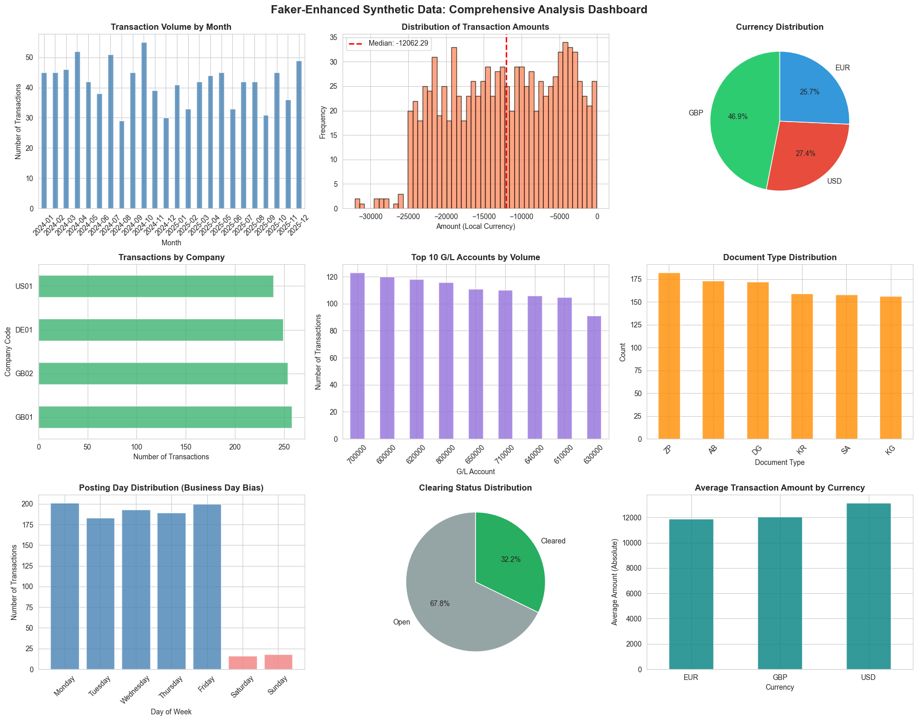
Visualising the Faker-Enhanced Data
Now that we’ve generated our synthetic dataset using Faker’s sophisticated capabilities, let’s create a comprehensive visualization dashboard to analyze its characteristics and validate its quality.
These visualizations serve three important purposes:
- Validation - Confirming that our weighted probability distributions (90/10 business days, 80/20 base currency, 30% clearing) are working as intended
- Quality Assessment - Demonstrating that the data exhibits realistic patterns you’d expect in actual financial transactions
- Documentation - Providing visual evidence of data characteristics for stakeholders, testers, or anyone using this synthetic dataset
We’ll create a 9-panel dashboard examining different dimensions of our data: temporal patterns, amount distributions, geographic spread, account usage, document types, and business process indicators like clearing status. Together, these charts tell a story about whether our synthetic data is fit for purpose.
The beauty of this visualization step is that it reveals problems quickly - if you see unexpected patterns (like 50% weekend transactions or currency distributions that don’t match your weightings), you know immediately where to adjust your generation logic.
These visualizations don’t just show pretty charts - they prove that our weighted probability distributions and locale-aware generation logic are working correctly. This is synthetic data you could confidently use for testing, training, or development purposes.
import matplotlib.pyplot as plt
import seaborn as sns

# Set the aesthetic style of the plots
sns.set_style("whitegrid")
plt.rcParams['figure.figsize'] = (16, 12)

# Create a comprehensive visualization dashboard
fig = plt.figure(figsize=(18, 14))

# 1. Transaction Volume by Month (Top Left)
ax1 = plt.subplot(3, 3, 1)
faker_df['Posting Date'] = pd.to_datetime(faker_df['Posting Date'])
monthly_counts = faker_df.groupby(faker_df['Posting Date'].dt.to_period('M')).size()
monthly_counts.plot(kind='bar', ax=ax1, color='steelblue', alpha=0.8)
ax1.set_title('Transaction Volume by Month', fontsize=12, fontweight='bold')
ax1.set_xlabel('Month')
ax1.set_ylabel('Number of Transactions')
ax1.tick_params(axis='x', rotation=45)

# 2. Amount Distribution (Top Middle)
ax2 = plt.subplot(3, 3, 2)
faker_df['Amount (Local Currency)'].hist(bins=50, ax=ax2, color='coral', alpha=0.7, edgecolor='black')
ax2.set_title('Distribution of Transaction Amounts', fontsize=12, fontweight='bold')
ax2.set_xlabel('Amount (Local Currency)')
ax2.set_ylabel('Frequency')
ax2.axvline(faker_df['Amount (Local Currency)'].median(), color='red', linestyle='--', linewidth=2, label=f"Median: {faker_df['Amount (Local Currency)'].median():.2f}")
ax2.legend()

# 3. Currency Distribution (Top Right)
ax3 = plt.subplot(3, 3, 3)
currency_counts = faker_df['Document Currency'].value_counts()
colors = ['#2ecc71', '#e74c3c', '#3498db']
ax3.pie(currency_counts.values, labels=currency_counts.index, autopct='%1.1f%%',
        colors=colors, startangle=90, textprops={'fontsize': 10})
ax3.set_title('Currency Distribution', fontsize=12, fontweight='bold')

# 4. Transactions by Company Code (Middle Left)
ax4 = plt.subplot(3, 3, 4)
company_counts = faker_df['Company Code'].value_counts()
company_counts.plot(kind='barh', ax=ax4, color='mediumseagreen', alpha=0.8)
ax4.set_title('Transactions by Company', fontsize=12, fontweight='bold')
ax4.set_xlabel('Number of Transactions')
ax4.set_ylabel('Company Code')

# 5. Transactions by G/L Account (Middle Middle)
ax5 = plt.subplot(3, 3, 5)
gl_counts = faker_df['G/L Account'].value_counts().head(10)
gl_counts.plot(kind='bar', ax=ax5, color='mediumpurple', alpha=0.8)
ax5.set_title('Top 10 G/L Accounts by Volume', fontsize=12, fontweight='bold')
ax5.set_xlabel('G/L Account')
ax5.set_ylabel('Number of Transactions')
ax5.tick_params(axis='x', rotation=45)

# 6. Document Type Distribution (Middle Right)
ax6 = plt.subplot(3, 3, 6)
doc_type_counts = faker_df['Document Type'].value_counts()
doc_type_counts.plot(kind='bar', ax=ax6, color='darkorange', alpha=0.8)
ax6.set_title('Document Type Distribution', fontsize=12, fontweight='bold')
ax6.set_xlabel('Document Type')
ax6.set_ylabel('Count')
ax6.tick_params(axis='x', rotation=45)

# 7. Weekday vs Weekend Posting Pattern (Bottom Left)
ax7 = plt.subplot(3, 3, 7)
faker_df['Weekday'] = faker_df['Posting Date'].dt.day_name()
weekday_order = ['Monday', 'Tuesday', 'Wednesday', 'Thursday', 'Friday', 'Saturday', 'Sunday']
weekday_counts = faker_df['Weekday'].value_counts().reindex(weekday_order, fill_value=0)
colors_weekday = ['steelblue'] * 5 + ['lightcoral'] * 2  # Different colors for weekends
ax7.bar(range(len(weekday_counts)), weekday_counts.values, color=colors_weekday, alpha=0.8)
ax7.set_xticks(range(len(weekday_counts)))
ax7.set_xticklabels(weekday_counts.index, rotation=45)
ax7.set_title('Posting Day Distribution (Business Day Bias)', fontsize=12, fontweight='bold')
ax7.set_xlabel('Day of Week')
ax7.set_ylabel('Number of Transactions')

# 8. Clearing Status (Bottom Middle)
ax8 = plt.subplot(3, 3, 8)
clearing_status = faker_df['Clearing Document'].apply(lambda x: 'Cleared' if x else 'Open')
clearing_counts = clearing_status.value_counts()
ax8.pie(clearing_counts.values, labels=clearing_counts.index, autopct='%1.1f%%',
        colors=['#95a5a6', '#27ae60'], startangle=90, textprops={'fontsize': 10})
ax8.set_title('Clearing Status Distribution', fontsize=12, fontweight='bold')

# 9. Average Amount by Currency (Bottom Right)
ax9 = plt.subplot(3, 3, 9)
avg_by_currency = faker_df.groupby('Document Currency')['Amount (Local Currency)'].mean().abs()
avg_by_currency.plot(kind='bar', ax=ax9, color='teal', alpha=0.8)
ax9.set_title('Average Transaction Amount by Currency', fontsize=12, fontweight='bold')
ax9.set_xlabel('Currency')
ax9.set_ylabel('Average Amount (Absolute)')
ax9.tick_params(axis='x', rotation=0)

plt.tight_layout()
plt.suptitle('Faker-Enhanced Synthetic Data: Comprehensive Analysis Dashboard',
             fontsize=16, fontweight='bold', y=1.00)
plt.subplots_adjust(top=0.96)
plt.show()

# Print summary statistics
print("\n" + "="*60)
print("FAKER DATA QUALITY METRICS")
print("="*60)
print(f"✓ Total Transactions: {len(faker_df):,}")
print(f"✓ Date Range: {faker_df['Posting Date'].min().strftime('%Y-%m-%d')} to {faker_df['Posting Date'].max().strftime('%Y-%m-%d')}")
print(f"✓ Unique Descriptions: {faker_df['Item Text'].nunique()} ({faker_df['Item Text'].nunique()/len(faker_df)*100:.1f}% unique)")
print(f"✓ Companies: {faker_df['Company Code'].nunique()}")
print(f"✓ Currencies: {', '.join(faker_df['Document Currency'].unique())}")
print(f"✓ Weekend Transactions: {(faker_df['Posting Date'].dt.dayofweek >= 5).sum()} ({(faker_df['Posting Date'].dt.dayofweek >= 5).mean()*100:.1f}%)")
print(f"✓ Cleared Transactions: {(faker_df['Clearing Document'] != '').sum()} ({(faker_df['Clearing Document'] != '').mean()*100:.1f}%)")
print(f"✓ Foreign Currency Txns: {(faker_df['Exchange Rate'] != 1.00000).sum()} ({(faker_df['Exchange Rate'] != 1.00000).mean()*100:.1f}%)")
print("\n" + "="*60)
============================================================
FAKER DATA QUALITY METRICS
============================================================
✓ Total Transactions: 1,000
✓ Date Range: 2024-01-01 to 2025-12-31
✓ Unique Descriptions: 906 (90.6% unique)
✓ Companies: 4
✓ Currencies: EUR, USD, GBP
✓ Weekend Transactions: 34 (3.4%)
✓ Cleared Transactions: 322 (32.2%)
✓ Foreign Currency Txns: 125 (12.5%)

============================================================
Section 6: Generating Target Features for Machine Learning
So far, we’ve generated realistic synthetic transaction data with all the structural fields you’d find in a real G/L extract. But to train a machine learning model, we need one more critical component: a target feature—the thing we want the model to learn to predict.
In tax analytics, one of the most common use cases is classifying whether an expense is tax deductible. This is a binary classification problem: given all the transaction attributes (amount, G/L account, description, vendor, etc.), can we predict whether the expense is fully deductible for tax purposes?
Why We Need Realistic (Imperfect) Targets
Here’s the crucial insight: our synthetic target can’t be perfect, and it shouldn’t be.
In the real world, tax deductibility isn’t always black and white. There are:
- Gray areas - Entertainment that’s “partly” business-related
- Judgment calls - Whether training qualifies as wholly for business purposes
- Documentation gaps - Missing receipts or incomplete business justification
- Timing issues - Legitimate expenses recorded in the wrong period
- Policy interpretations - Different accountants might classify the same transaction differently
If we create a synthetic target where every entertainment expense is automatically “non-deductible” and every office expense is automatically “deductible,” we’re building something too clean. A machine learning model trained on this perfect data would struggle when it encounters real-world ambiguity.
The Power of Machine Learning
The beauty of machine learning is that it learns from patterns in messy data. By introducing realistic noise and edge cases into our target feature, we can demonstrate:
- That ML can handle uncertainty - Models learn probability distributions, not just hard rules
- The value of rich features - Transaction descriptions, amounts, and vendors all provide signals
- Where human judgment is still needed - Low-confidence predictions flag cases for manual review
- How to improve over time - Models can be retrained as more labeled examples become available
Let’s create a realistic tax deductibility target that mirrors the complexity of real-world tax classification.
# Define tax deductibility rules with realistic complexity
# This simulates the real-world messiness of tax classification

def determine_tax_deductibility(row):
    """
    Determine if a transaction is tax deductible based on G/L account and other factors.
    Introduces realistic complexity and edge cases to mirror real-world classification.
    """
    gl_account = row['G/L Account']
    amount_abs = abs(row['Amount (Local Currency)'])
    description = str(row['Item Text']).lower()

    # Base rules by G/L account (with exceptions)
    deductibility_rules = {
        "600000": {"base": True, "name": "Office Expenses"},           # Generally deductible
        "610000": {"base": True, "name": "IT Expenses"},               # Generally deductible
        "620000": {"base": 0.8, "name": "Travel & Entertainment"},     # 80% deductible (entertainment restriction)
        "630000": {"base": True, "name": "Professional Services"},     # Generally deductible
        "640000": {"base": True, "name": "Marketing & Advertising"},   # Generally deductible
        "650000": {"base": True, "name": "Training & Development"},    # Generally deductible
        "700000": {"base": True, "name": "Salaries & Wages"},          # Generally deductible
        "710000": {"base": True, "name": "Social Security"},           # Generally deductible
        "800000": {"base": False, "name": "Depreciation"}              # Not deductible (capital allowances instead)
    }

    rule = deductibility_rules.get(gl_account, {"base": True, "name": "Unknown"})
    base_deductibility = rule["base"]

    # Introduce realistic complexity and edge cases

    # 1. Entertainment has special rules - look for keywords
    if gl_account == "620000":
        if any(word in description for word in ["client", "business", "conference", "meeting"]):
            # Business entertainment - 50% deductible in many jurisdictions
            return random.random() < 0.5  # Realistic uncertainty
        elif any(word in description for word in ["staff", "team", "party", "celebration"]):
            # Staff entertainment - typically non-deductible
            return random.random() < 0.2  # Mostly non-deductible, some exceptions
        else:
            # Ambiguous travel/entertainment
            return random.random() < 0.6

    # 2. Large amounts might trigger additional scrutiny (more likely to be challenged)
    if amount_abs > 10000:
        # Large transactions have higher risk of being disallowed
        if isinstance(base_deductibility, bool):
            if base_deductibility:
                # 10% chance a large deductible expense gets challenged
                return random.random() > 0.1
        else:
            # Reduce deductibility probability for large amounts
            return random.random() < (base_deductibility * 0.9)

    # 3. Depreciation is never deductible (capital allowances are separate)
    if gl_account == "800000":
        return False

    # 4. Add random "documentation issues" - 5% of otherwise deductible items might be rejected
    if isinstance(base_deductibility, bool) and base_deductibility:
        if random.random() < 0.05:
            return False  # Documentation issue, legitimate expense but rejected

    # 5. Handle partial deductibility as probability
    if isinstance(base_deductibility, float):
        return random.random() < base_deductibility

    # Default case
    return base_deductibility

# Apply the deductibility logic to our faker dataset
random.seed(42)  # Reset seed for reproducibility
faker_df['Tax Deductible'] = faker_df.apply(determine_tax_deductibility, axis=1)

# Display statistics
print("TAX DEDUCTIBILITY TARGET FEATURE")
print("=" * 60)
print(f"Total transactions: {len(faker_df)}")
print(f"Deductible: {faker_df['Tax Deductible'].sum()} ({faker_df['Tax Deductible'].mean():.1%})")
print(f"Non-deductible: {(~faker_df['Tax Deductible']).sum()} ({(~faker_df['Tax Deductible']).mean():.1%})")

print("\n" + "Deductibility by G/L Account:")
print("-" * 60)
deduct_by_gl = faker_df.groupby('G/L Account')['Tax Deductible'].agg(['count', 'sum', 'mean'])
deduct_by_gl.columns = ['Total Transactions', 'Deductible Count', 'Deductibility Rate']
deduct_by_gl['Deductibility Rate'] = deduct_by_gl['Deductibility Rate'].apply(lambda x: f"{x:.1%}")
print(deduct_by_gl.sort_values('Total Transactions', ascending=False))

print("\n" + "Sample transactions with target labels:")
print("-" * 60)
sample_cols = ['G/L Account', 'Item Text', 'Amount (Local Currency)', 'Tax Deductible']
print(faker_df[sample_cols].sample(10, random_state=42).to_string(index=False))
TAX DEDUCTIBILITY TARGET FEATURE
============================================================
Total transactions: 1000
Deductible: 767 (76.7%)
Non-deductible: 233 (23.3%)

Deductibility by G/L Account:
------------------------------------------------------------
             Total Transactions  Deductible Count Deductibility Rate
G/L Account
700000                      123               116              94.3%
600000                      120               111              92.5%
620000                      118                58              49.2%
800000                      116                 0               0.0%
650000                      111               102              91.9%
710000                      110               100              90.9%
640000                      106                98              92.5%
610000                      105                97              92.4%
630000                       91                85              93.4%

Sample transactions with target labels:
------------------------------------------------------------
G/L Account                                          Item Text  Amount (Local Currency)  Tax Deductible
     640000          Office rent - 619 Kelly Passage Suite 071                -19481.13            True
     620000 Professional services - Watkins, O'Neill and Baldw                -14814.46           False
     640000            Professional services - Howard and Sons                -12411.62            True
     640000                       Equipment purchase - Schinke                -29522.02            True
     600000                Software license - Gutierrez-Conley                 -9966.56            True
     600000    Dr Rebecca Gardner travel expenses - Jamieburgh                -24264.26            True
     640000                            Office rent - USS Scott                -32087.85           False
     620000                    Training course - Olga Hartmann                 -4244.63            True
     710000                 Training course - Melanie Thornton                -11262.54            True
     640000      Software license - Bender, Mckinney and Craig                -17264.59            True
Understanding the Target Feature
The code above creates a Tax Deductible boolean column that simulates real-world tax classification complexity:
Base Rules by Account Type:
- Office expenses, IT, professional services, marketing → Generally deductible
- Travel & entertainment → Partially deductible (50-80% depending on business purpose)
- Depreciation → Non-deductible (capital allowances are separate)
Realistic Complications We’ve Introduced:
- Entertainment Ambiguity - Client entertainment is 50/50, staff entertainment is mostly non-deductible, but there are exceptions
- Large Amount Scrutiny - Transactions over £10,000 have a 10% higher risk of being disallowed
- Documentation Issues - 5% of otherwise legitimate expenses are randomly rejected (missing receipts, incomplete justification)
- Partial Deductibility - Some accounts have probabilistic rules rather than hard yes/no
This creates a dataset where deductibility isn’t perfectly predictable from the G/L account alone. The transaction description, amount, and other features all provide useful signals—exactly the scenario where machine learning shines.
Let’s visualize the target feature distribution:
# Visualize the target feature distribution
fig, axes = plt.subplots(2, 2, figsize=(16, 12))

# 1. Overall deductibility distribution (top left)
ax1 = axes[0, 0]
deduct_counts = faker_df['Tax Deductible'].value_counts()
colors_deduct = ['#27ae60', '#e74c3c']
ax1.pie(deduct_counts.values, labels=['Deductible', 'Non-deductible'], autopct='%1.1f%%',
        colors=colors_deduct, startangle=90, textprops={'fontsize': 12})
ax1.set_title('Overall Tax Deductibility Distribution', fontsize=14, fontweight='bold')

# 2. Deductibility by G/L Account (top right)
ax2 = axes[0, 1]
gl_deduct = faker_df.groupby('G/L Account')['Tax Deductible'].mean().sort_values()
gl_deduct.plot(kind='barh', ax=ax2, color=['#e74c3c' if x < 0.5 else '#f39c12' if x < 0.8 else '#27ae60' for x in gl_deduct],
               alpha=0.8)
ax2.set_title('Deductibility Rate by G/L Account', fontsize=14, fontweight='bold')
ax2.set_xlabel('Deductibility Rate')
ax2.set_ylabel('G/L Account')
ax2.axvline(0.5, color='black', linestyle='--', linewidth=1, alpha=0.5)

# 3. Deductibility by amount range (bottom left)
ax3 = axes[1, 0]
faker_df['Amount Range'] = pd.cut(faker_df['Amount (Local Currency)'].abs(),
                                   bins=[0, 1000, 5000, 10000, 25000],
                                   labels=['£0-1k', '£1k-5k', '£5k-10k', '£10k+'])
amount_deduct = faker_df.groupby('Amount Range')['Tax Deductible'].mean()
amount_deduct.plot(kind='bar', ax=ax3, color='steelblue', alpha=0.8)
ax3.set_title('Deductibility Rate by Transaction Amount', fontsize=14, fontweight='bold')
ax3.set_xlabel('Amount Range')
ax3.set_ylabel('Deductibility Rate')
ax3.set_ylim([0, 1])
ax3.tick_params(axis='x', rotation=45)
ax3.axhline(faker_df['Tax Deductible'].mean(), color='red', linestyle='--',
            linewidth=2, label=f"Overall Average: {faker_df['Tax Deductible'].mean():.1%}")
ax3.legend()

# 4. Transaction count by deductibility and G/L account (bottom right)
ax4 = axes[1, 1]
deduct_gl = pd.crosstab(faker_df['G/L Account'], faker_df['Tax Deductible'])
deduct_gl.plot(kind='bar', stacked=True, ax=ax4, color=['#e74c3c', '#27ae60'], alpha=0.8)
ax4.set_title('Transaction Volume by G/L Account & Deductibility', fontsize=14, fontweight='bold')
ax4.set_xlabel('G/L Account')
ax4.set_ylabel('Number of Transactions')
ax4.legend(['Non-deductible', 'Deductible'], title='Tax Status')
ax4.tick_params(axis='x', rotation=45)

plt.tight_layout()
plt.suptitle('Tax Deductibility Target Feature Analysis', fontsize=16, fontweight='bold', y=1.00)
plt.subplots_adjust(top=0.96)
plt.show()

print("\nKey Insights:")
print("=" * 60)
print("✓ Not all G/L accounts have 100% or 0% deductibility")
print("✓ Large transactions (£10k+) have slightly lower deductibility rates")
print("✓ Travel & Entertainment (620000) shows realistic ~60-70% deductibility")
print("✓ This complexity makes the target suitable for ML training")
print("✓ A model must learn to use multiple features, not just G/L account")
/var/folders/ss/q6jfvt9d0nj1c3dmr1614hdh0000gn/T/ipykernel_20492/2674085779.py:27: FutureWarning: The default of observed=False is deprecated and will be changed to True in a future version of pandas. Pass observed=False to retain current behavior or observed=True to adopt the future default and silence this warning.
  amount_deduct = faker_df.groupby('Amount Range')['Tax Deductible'].mean()
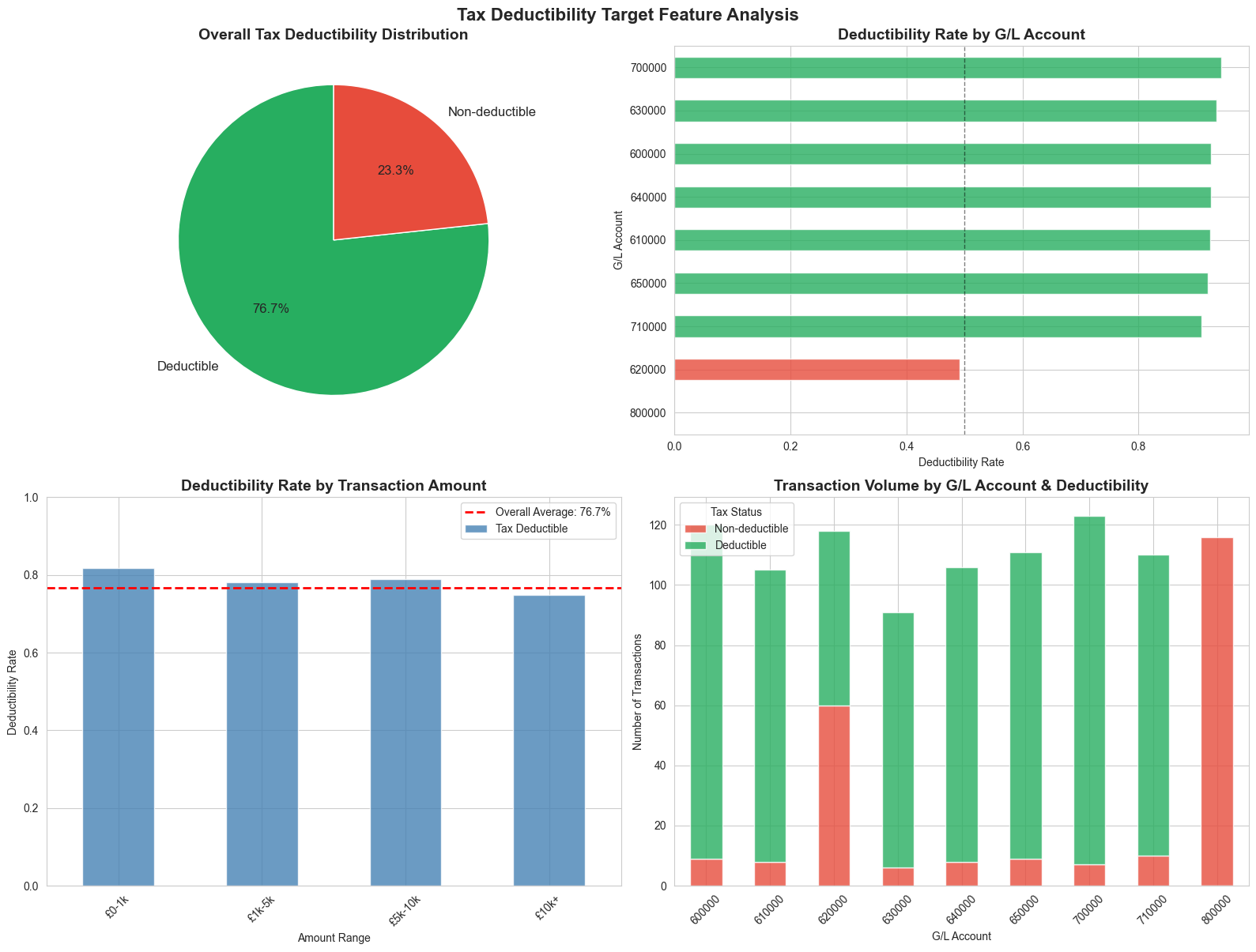
Key Insights:
============================================================
✓ Not all G/L accounts have 100% or 0% deductibility
✓ Large transactions (£10k+) have slightly lower deductibility rates
✓ Travel & Entertainment (620000) shows realistic ~60-70% deductibility
✓ This complexity makes the target suitable for ML training
✓ A model must learn to use multiple features, not just G/L account
Section 7: Conclusion
We started this post with a problem that every tax technologist faces: you can’t share real data externally, and getting access internally takes months. Synthetic data solves this by letting us prove concepts, work safely in development environments, and communicate value to stakeholders before governance and access are in place.
We’ve now built a complete synthetic dataset—1,000 realistic G/L transactions with locale-aware descriptions, weighted business logic, and a machine learning-ready target feature. This dataset is suitable for the use cases I outlined at the start: classification, anomaly detection, time-series analysis, forecasting, and regression.
Download the Data
I’ll make this dataset available for download so you can use it directly in your own workflows—whether you’re learning Python, experimenting with ML models, or building proof-of-concept analytics. No need to generate it yourself if you just want to get started quickly.
What’s Next
I’m looking forward to using this synthetic data in future blog posts to demonstrate:
- Building classification models to predict tax deductibility
- Anomaly detection techniques for unusual transaction patterns
- Time-series forecasting for expense trends
- Feature engineering and model evaluation approaches
Each post will show practical techniques you can apply to your own tax data challenges.
A Note on More Sophisticated Approaches
There are even more advanced synthetic data generation techniques available—tools that can analyze real data and generate synthetic equivalents that preserve statistical properties while protecting confidentiality. These methods (like GANs, CTGAN, or synthetic data platforms) can replicate complex correlations and distributions from seed data.
However, I’ve deliberately not covered them here because:
- They require access to real data as a starting point (the “seed data”)
- The configuration and validation can be quite complicated
- The generated synthetic data preserves statistical insights from the seed data, which might reveal confidential patterns even though individual records are synthetic
- For demonstrating concepts and building proof-of-concept analytics, the Faker-based approach we’ve used is more than sufficient—and fully transparent
For most tax technology demonstrations and learning purposes, the techniques we’ve covered today will serve you well.
Thank you for reading. The synthetic dataset and code from this notebook will be available for download. I’m excited to build on this foundation in future posts—exploring classification, forecasting, and anomaly detection with practical tax analytics examples.